Tidy data
Whenever we start our journey transforming a dataset into an organized format we can interpret and visualize, it helps to to have the data in Tidy format. Tidy data is a structure for data sets that helps R do the most work possible when it comes to analysis, summary statistics, and combining data sets. R’s vectorized functions flourish with rows and columns in Tidy format.
Tidy data has each variable in columns, each observation has its own row, and each cell contains a single value. For the lobster data set, each lobster caught has its own row with each column describing one aspect of that lobster. Each column has a succinct title for the variable it contains, and ideally includes underscores where we would normally have spaces and has no capitalization to make our coding as easy as possible. There should be NA in any cells that do not have values, which is a default that many R functions recognize as default. When we utilize this data, we can easily remove these values in our code by referring to them as NA.
Tidy format encourages collaboration between people and data sets because we are easily able to combine data from different sources using join functions. If the data contains columns with shared variables, R can easily recognize those columns and associate its rows (observations) with the observations of the complementary data set. Using full_join() is a common join function to utilize as it maintains all data from both sources.
Tidy format helps you easily make subsets of your data for specific graphs and summary tables. Consider the filter() and select() functions, which help you subset to only view variable or observations of interest. In these cases, it is especially important to have only one value in each cell and standardize the way you document observations. You always want to record each lobster species with the same spelling, each size with the same number of decimal places, and each date with the same format (such as YYYY-MM-DD). For variables such as length that might need units, always include these units in the column header rather than the cell. This streamlines our coding and keeps cells to a single class. If you include numerical and character values in one cell, it will be documented as a character, which can restrict your analysis process.
Your data isn’t in Tidy format? That’s alright! Check out the tidyr::pivot_longer() and tidyr::pivot_wider() functions to help you help R help you. In the example below, we have a tribble dataset that is not in Tidy format. We know this because there are multiple columns (A:C) that represent different individuals or observations of the same variable (like dog food brands). We can use pivot_longer() to put the column headers into their own column, rename that column, and pivot their values into their own column while maintaining their association with A, B, and C. Although the resulting tidy data may seem more complex at first galnce, it is easier to convert to a graph and structurally is more organized from a data science perspective.
To demonstrate some simple data tidying, lets make a tribble (which is similar to a dataframe) and manipulate it using the pivot_longer() function. In this example tibble, we are comparing the food preferences of 2 dogs. The dog food types are labeled as A, B, and C.
df <- tribble(
  ~name, ~A, ~B, ~C,
  "dog_1", 4, 5, 6,
  "dog_2", 9, 10, 8
)

df
# A tibble: 2 × 4
  name      A     B     C
  <chr> <dbl> <dbl> <dbl>
1 dog_1     4     5     6
2 dog_2     9    10     8
This dataframe is not in tidy format, because the variable ranking is dispersed between multiple columns. We want a single variable in each column, so lets combine those columns and make it tidier:
# A tibble: 6 × 3
  name  dog_food_brand ranking
  <chr> <chr>            <dbl>
1 dog_1 A                    4
2 dog_1 B                    5
3 dog_1 C                    6
4 dog_2 A                    9
5 dog_2 B                   10
6 dog_2 C                    8
Wonderful, now let’s apply these Tidy tools to a substantial dataset!
case_when() and Lobster Data
First thing first, import your data
# A tibble: 6 × 9
   year month date       site  transect replicate size_mm num_ao  area
  <dbl> <dbl> <date>     <chr>    <dbl> <chr>       <dbl>  <dbl> <dbl>
1  2012     8 2012-08-20 IVEE         3 A              70      0   300
2  2012     8 2012-08-20 IVEE         3 B              60      0   300
3  2012     8 2012-08-20 IVEE         3 B              65      0   300
4  2012     8 2012-08-20 IVEE         3 B              70      0   300
5  2012     8 2012-08-20 IVEE         3 B              85      0   300
6  2012     8 2012-08-20 IVEE         3 C              60      0   300
Use the case_when() function to tidy this lobster data and prepare it for visualization. The case_when() function bins continuous data into manually defined categories and adds this categorization it to your data set in the form of new column. It doesn’t change the values in the cells that already exist, and it does not delete any existing data.
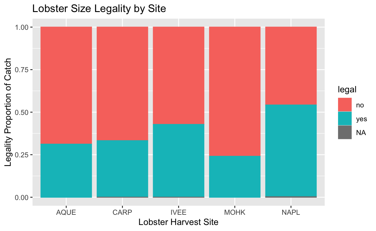
Lobsters must be a minimum size in order to harvest, and we can use case_when() to categorize lobsters into size bins based on the legal size minimum for fishing. This function processes each individual lobster (each row) in this dataframe and returns if it is large enough to legally harvest from various locations along the Santa Barbara coast.
This data is ground-breaking! The world needs to see this and understand its implications. In order to plot this fascinating data in a meaningful way, we want to efficiently categorize our lobsters by legality status and color code their relative abundance in our visualization. Considering that the legal minimum size for a lobster is 79.76 (units), this is the threshold we will pass onto R to do the heavy lifting for us.
Use ggplot() to make a bar graph that color codes the lobster abundance by legality status. We communicate that we want R to color the graph by this variable by passing the argument color = legal within aes(). Manually setting colors is set outside of aes(), but here it is an argument because it is determined by a variable.
Distill is a publication format for scientific and technical writing, native to the web. Learn more about using Distill at https://rstudio.github.io/distill.